Compute Graph properties from a given connectivity matrix with BCT toolbox¶

The conmat_to_graph pipeline provide an example wrap of a function from the bctpy toolbox (Brain Connectivity Toolbox) <https://sites.google.com/site/bctnet/> as an alternative to the Radatools toolbox for graph metric computation.

The input data should be a symetrical connecivity matrix in npy format.

# Authors: David Meunier <david_meunier_79@hotmail.fr>

# License: BSD (3-clause)
# sphinx_gallery_thumbnail_number = 2
import os.path as op

import nipype.pipeline.engine as pe

from nipype.interfaces.utility import IdentityInterface
import nipype.interfaces.io as nio

Check if data are available

from graphpype.utils_tests import load_test_data

data_path = load_test_data("data_con_meg")

This will be what we will loop on

freq_band_names = ['alpha', 'beta']

Then, we create our workflow and specify the base_dir which tells nipype the directory in which to store the outputs.

# workflow directory within the `base_dir`
graph_analysis_name = 'graph_analysis'

main_workflow = pe.Workflow(name=graph_analysis_name)
main_workflow.base_dir = data_path

Then we create a node to pass input filenames to DataGrabber from nipype

infosource = pe.Node(
        interface=IdentityInterface(fields=['freq_band_name']),
        name="infosource")

infosource.iterables = [('freq_band_name', freq_band_names)]

and a node to grab data. The template_args in this node iterate upon the values in the infosource node

# template_path = '*%s/conmat_0_coh.npy'
# template_args = [['freq_band_name']
# datasource = create_datagrabber(data_path, template_path, template_args)

datasource = pe.Node(
    interface=nio.DataGrabber(infields=['freq_band_name'],
                              outfields=['conmat_file']),
    name='datasource')
datasource.inputs.base_directory = data_path
datasource.inputs.template = ("%s/conmat_0_coh.npy")
datasource.inputs.template_args = dict(
    conmat_file=[['freq_band_name']])

datasource.inputs.sort_filelist = True

This parameter corrdesponds to the percentage of highest connections retains for the analyses. con_den = 1.0 means a fully connected graphs (all edges are present)

import json  # noqa
import pprint  # noqa

data_graph = json.load(open(op.join(op.dirname("__file__"),
                                  "params_bct_graph.json")))
pprint.pprint({'graph parameters': data_graph})

# density of the threshold
con_den = data_graph['con_den']


from graphpype.pipelines import create_pipeline_bct_graph

graph_workflow = create_pipeline_bct_graph(
    data_path, con_den=con_den)

Out:

{'graph parameters': {'con_den': 0.05}}

We then connect the nodes two at a time. We connect the output of the infosource node to the datasource node. So, these two nodes taken together can grab data.

main_workflow.connect(infosource, 'freq_band_name',
                      datasource, 'freq_band_name')

main_workflow.connect(datasource, 'conmat_file',
                      graph_workflow, "inputnode.conmat_file")

To do so, we first write the workflow graph (optional)

main_workflow.write_graph(graph2use='colored')  # colored

and visualize it. Take a moment to pause and notice how the connections here correspond to how we connected the nodes.

#import matplotlib.pyplot as plt  # noqa
#img = plt.imread(op.join(data_path, graph_analysis_name, 'graph.png'))
#plt.figure(figsize=(8, 8))
#plt.imshow(img)
#plt.axis('off')
#plt.show()

Finally, we are now ready to execute our workflow.

main_workflow.config['execution'] = {'remove_unnecessary_outputs': 'false'}

# Run workflow locally on 2 CPUs
main_workflow.run(plugin='MultiProc', plugin_args={'n_procs': 2})

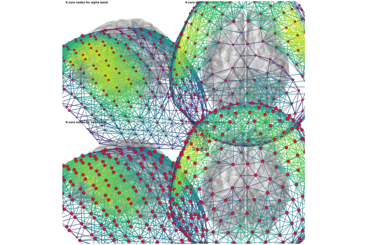
plotting k_core values

from graphpype.utils_visbrain import visu_graph # noqa

labels_file = op.join(data_path, "correct_channel_names.txt")
coords_file = op.join(data_path, "MNI_coords.txt")

#labels_file = op.join(data_path, "label_names.txt")
#coords_file = op.join(data_path, "label_centroid.txt")

from visbrain.objects import SceneObj, BrainObj # noqa

sc = SceneObj(size=(1500, 1500), bgcolor=(1,1,1))

views = ["left",'top']


for nf, freq_band_name in enumerate(freq_band_names):

    res_path = op.join(
        data_path, graph_analysis_name,
        "graph_bct_pipe",
        "_freq_band_name_"+freq_band_name)

    node_k_file = op.join(res_path, "k_core", "coreness.npy")

    bin_mat_file = op.join(res_path, "bin_mat", "bin_mat.npy")

    for i_v,view in enumerate(views):
        b_obj = BrainObj('B1', translucent=True)

        sc.add_to_subplot(b_obj, row=nf, col = i_v, use_this_cam=True, rotate=view,
                        title=("K-core nodes for {} band".format(freq_band_name)),
                        title_size=14, title_bold=True, title_color='black')

        c_obj,s_obj = visu_graph(
            labels_file = labels_file, coords_file = coords_file,
            #net_file = bin_mat_file)
            net_file = bin_mat_file, node_size_file=node_k_file)

        sc.add_to_subplot(c_obj, row=nf, col = i_v)
        sc.add_to_subplot(s_obj, row=nf, col = i_v)

sc.preview()

../_images/sphx_glr_plot_conmat_to_bct_graph_001.png

Out:

.npy
[[0 1 1 ... 0 0 0]
 [0 0 1 ... 0 0 0]
 [0 0 0 ... 0 0 0]
 ...
 [0 0 0 ... 0 0 0]
 [0 0 0 ... 0 0 0]
 [0 0 0 ... 0 0 0]]
[[-- 1 1 ... -- -- --]
 [-- -- 1 ... -- -- --]
 [-- -- -- ... -- -- --]
 ...
 [-- -- -- ... -- -- --]
 [-- -- -- ... -- -- --]
 [-- -- -- ... -- -- --]]
(270, 270) (270, 3) (270,)
[3. 2. 2. 2. 2. 2. 2. 2. 2. 2. 2. 2. 2. 2. 2. 2. 2. 2. 2. 2. 2. 2. 2. 2.
 2. 2. 2. 2. 2. 2. 2. 2. 2. 2. 2. 2. 2. 2. 2. 2. 2. 2. 2. 2. 2. 2. 2. 2.
 2. 2. 2. 2. 2. 2. 2. 2. 2. 2. 2. 2. 2. 2. 2. 1. 2. 2. 2. 1. 2. 2. 2. 2.
 2. 2. 1. 2. 2. 2. 2. 2. 2. 2. 2. 2. 2. 2. 2. 2. 2. 2. 2. 1. 1. 1. 2. 2.
 2. 2. 2. 2. 2. 2. 2. 2. 2. 2. 2. 2. 1. 1. 1. 1. 1. 2. 1. 2. 1. 1. 1. 1.
 1. 1. 1. 1. 1. 1. 1. 1. 1. 1. 0. 3. 2. 2. 2. 2. 2. 2. 2. 2. 2. 2. 2. 2.
 2. 2. 2. 2. 2. 2. 2. 2. 2. 2. 2. 2. 2. 2. 2. 2. 2. 2. 2. 2. 2. 2. 2. 2.
 2. 2. 2. 2. 2. 2. 2. 2. 2. 2. 2. 2. 2. 2. 2. 2. 2. 2. 2. 2. 2. 2. 2. 2.
 2. 2. 2. 2. 2. 2. 2. 2. 2. 2. 2. 2. 2. 2. 1. 2. 2. 2. 2. 2. 2. 2. 2. 2.
 2. 1. 1. 2. 2. 2. 1. 1. 1. 2. 2. 2. 2. 2. 2. 2. 2. 2. 2. 2. 2. 2. 2. 2.
 1. 2. 2. 2. 2. 1. 1. 1. 1. 1. 1. 1. 1. 1. 0. 1. 1. 1. 0. 0. 0. 1. 1. 0.
 1. 0. 1. 0. 0. 0.]
.npy
[[0 1 1 ... 0 0 0]
 [0 0 1 ... 0 0 0]
 [0 0 0 ... 0 0 0]
 ...
 [0 0 0 ... 0 0 0]
 [0 0 0 ... 0 0 0]
 [0 0 0 ... 0 0 0]]
[[-- 1 1 ... -- -- --]
 [-- -- 1 ... -- -- --]
 [-- -- -- ... -- -- --]
 ...
 [-- -- -- ... -- -- --]
 [-- -- -- ... -- -- --]
 [-- -- -- ... -- -- --]]
(270, 270) (270, 3) (270,)
[3. 2. 2. 2. 2. 2. 2. 2. 2. 2. 2. 2. 2. 2. 2. 2. 2. 2. 2. 2. 2. 2. 2. 2.
 2. 2. 2. 2. 2. 2. 2. 2. 2. 2. 2. 2. 2. 2. 2. 2. 2. 2. 2. 2. 2. 2. 2. 2.
 2. 2. 2. 2. 2. 2. 2. 2. 2. 2. 2. 2. 2. 2. 2. 1. 2. 2. 2. 1. 2. 2. 2. 2.
 2. 2. 1. 2. 2. 2. 2. 2. 2. 2. 2. 2. 2. 2. 2. 2. 2. 2. 2. 1. 1. 1. 2. 2.
 2. 2. 2. 2. 2. 2. 2. 2. 2. 2. 2. 2. 1. 1. 1. 1. 1. 2. 1. 2. 1. 1. 1. 1.
 1. 1. 1. 1. 1. 1. 1. 1. 1. 1. 0. 3. 2. 2. 2. 2. 2. 2. 2. 2. 2. 2. 2. 2.
 2. 2. 2. 2. 2. 2. 2. 2. 2. 2. 2. 2. 2. 2. 2. 2. 2. 2. 2. 2. 2. 2. 2. 2.
 2. 2. 2. 2. 2. 2. 2. 2. 2. 2. 2. 2. 2. 2. 2. 2. 2. 2. 2. 2. 2. 2. 2. 2.
 2. 2. 2. 2. 2. 2. 2. 2. 2. 2. 2. 2. 2. 2. 1. 2. 2. 2. 2. 2. 2. 2. 2. 2.
 2. 1. 1. 2. 2. 2. 1. 1. 1. 2. 2. 2. 2. 2. 2. 2. 2. 2. 2. 2. 2. 2. 2. 2.
 1. 2. 2. 2. 2. 1. 1. 1. 1. 1. 1. 1. 1. 1. 0. 1. 1. 1. 0. 0. 0. 1. 1. 0.
 1. 0. 1. 0. 0. 0.]
.npy
[[0 1 1 ... 0 0 0]
 [0 0 1 ... 0 0 0]
 [0 0 0 ... 0 0 0]
 ...
 [0 0 0 ... 0 0 0]
 [0 0 0 ... 0 0 0]
 [0 0 0 ... 0 0 0]]
[[-- 1 1 ... -- -- --]
 [-- -- 1 ... -- -- --]
 [-- -- -- ... -- -- --]
 ...
 [-- -- -- ... -- -- --]
 [-- -- -- ... -- -- --]
 [-- -- -- ... -- -- --]]
(270, 270) (270, 3) (270,)
[2. 2. 2. 2. 2. 2. 2. 2. 2. 2. 2. 2. 2. 2. 2. 2. 2. 2. 2. 2. 2. 2. 2. 2.
 2. 2. 2. 2. 2. 2. 2. 2. 2. 2. 2. 2. 2. 2. 2. 2. 2. 2. 2. 2. 2. 2. 2. 2.
 2. 2. 2. 2. 2. 2. 2. 2. 2. 2. 2. 2. 2. 2. 2. 2. 2. 2. 2. 2. 2. 2. 2. 2.
 1. 1. 1. 2. 2. 2. 2. 2. 2. 2. 2. 2. 2. 2. 2. 2. 2. 2. 2. 1. 1. 1. 2. 2.
 2. 2. 2. 2. 2. 2. 2. 2. 2. 2. 2. 2. 2. 2. 2. 2. 2. 2. 2. 2. 1. 2. 2. 2.
 1. 1. 1. 1. 1. 1. 1. 1. 1. 1. 0. 2. 2. 2. 2. 2. 2. 2. 2. 2. 2. 2. 2. 2.
 2. 2. 2. 2. 2. 2. 2. 2. 2. 2. 2. 2. 2. 2. 2. 2. 2. 2. 2. 2. 2. 2. 2. 2.
 2. 2. 2. 2. 2. 2. 2. 2. 2. 2. 2. 2. 2. 2. 2. 2. 2. 2. 2. 2. 2. 2. 2. 2.
 2. 2. 2. 2. 2. 2. 2. 2. 2. 2. 2. 2. 2. 2. 1. 2. 2. 2. 2. 2. 2. 2. 2. 2.
 2. 2. 2. 2. 2. 2. 1. 1. 1. 2. 2. 2. 2. 2. 2. 2. 2. 2. 2. 2. 2. 2. 2. 2.
 1. 2. 2. 2. 2. 1. 1. 2. 2. 1. 1. 1. 1. 1. 0. 1. 1. 1. 0. 1. 0. 1. 1. 0.
 1. 0. 1. 0. 0. 0.]
.npy
[[0 1 1 ... 0 0 0]
 [0 0 1 ... 0 0 0]
 [0 0 0 ... 0 0 0]
 ...
 [0 0 0 ... 0 0 0]
 [0 0 0 ... 0 0 0]
 [0 0 0 ... 0 0 0]]
[[-- 1 1 ... -- -- --]
 [-- -- 1 ... -- -- --]
 [-- -- -- ... -- -- --]
 ...
 [-- -- -- ... -- -- --]
 [-- -- -- ... -- -- --]
 [-- -- -- ... -- -- --]]
(270, 270) (270, 3) (270,)
[2. 2. 2. 2. 2. 2. 2. 2. 2. 2. 2. 2. 2. 2. 2. 2. 2. 2. 2. 2. 2. 2. 2. 2.
 2. 2. 2. 2. 2. 2. 2. 2. 2. 2. 2. 2. 2. 2. 2. 2. 2. 2. 2. 2. 2. 2. 2. 2.
 2. 2. 2. 2. 2. 2. 2. 2. 2. 2. 2. 2. 2. 2. 2. 2. 2. 2. 2. 2. 2. 2. 2. 2.
 1. 1. 1. 2. 2. 2. 2. 2. 2. 2. 2. 2. 2. 2. 2. 2. 2. 2. 2. 1. 1. 1. 2. 2.
 2. 2. 2. 2. 2. 2. 2. 2. 2. 2. 2. 2. 2. 2. 2. 2. 2. 2. 2. 2. 1. 2. 2. 2.
 1. 1. 1. 1. 1. 1. 1. 1. 1. 1. 0. 2. 2. 2. 2. 2. 2. 2. 2. 2. 2. 2. 2. 2.
 2. 2. 2. 2. 2. 2. 2. 2. 2. 2. 2. 2. 2. 2. 2. 2. 2. 2. 2. 2. 2. 2. 2. 2.
 2. 2. 2. 2. 2. 2. 2. 2. 2. 2. 2. 2. 2. 2. 2. 2. 2. 2. 2. 2. 2. 2. 2. 2.
 2. 2. 2. 2. 2. 2. 2. 2. 2. 2. 2. 2. 2. 2. 1. 2. 2. 2. 2. 2. 2. 2. 2. 2.
 2. 2. 2. 2. 2. 2. 1. 1. 1. 2. 2. 2. 2. 2. 2. 2. 2. 2. 2. 2. 2. 2. 2. 2.
 1. 2. 2. 2. 2. 1. 1. 2. 2. 1. 1. 1. 1. 1. 0. 1. 1. 1. 0. 1. 0. 1. 1. 0.
 1. 0. 1. 0. 0. 0.]

Total running time of the script: ( 0 minutes 12.861 seconds)

Gallery generated by Sphinx-Gallery