Compute PSD on sensor space

The power pipeline computes the power spectral density (PSD) on epochs or raw data on sensor space or source space. The mean PSD for each selected frequency band is also computed and saved in a numpy file.

The input data shoud be in fif or numpy format.

# Authors: Annalisa Pascarella <a.pascarella@iac.cnr.it>
#          Mainak Jas <mainakjas@gmail.com>
# License: BSD (3-clause)

# sphinx_gallery_thumbnail_number = 2

import os.path as op
import numpy as np
import nipype.pipeline.engine as pe

import ephypype
from ephypype.nodes import create_iterator, create_datagrabber
from ephypype.datasets import fetch_omega_dataset

Let us fetch the data first. It is around 675 MB download.

base_path = op.join(op.dirname(ephypype.__file__), '..', 'examples')
data_path = fetch_omega_dataset(base_path)

then read the parameters for experiment and power analysis from a json file and print it

import json  # noqa
import pprint  # noqa
params = json.load(open("params.json"))

pprint.pprint({'experiment parameters': params["general"]})
subject_ids = params["general"]["subject_ids"]  # sub-003
session_ids = params["general"]["session_ids"]  # ses-0001
NJOBS = params["general"]["NJOBS"]

pprint.pprint({'power parameters': params["power"]})
freq_band_names = params["power"]['freq_band_names']
freq_bands = params["power"]['freq_bands']
is_epoched = params["power"]['is_epoched']
fmin = params["power"]['fmin']
fmax = params["power"]['fmax']
power_method = params["power"]['method']

{'experiment parameters': {'NJOBS': 1,
                           'data_type': 'fif',
                           'session_ids': ['ses-0001'],
                           'subject_ids': ['sub-0003'],
                           'subjects_dir': 'FSF'}}
{'power parameters': {'fmax': 150,
                      'fmin': 0.1,
                      'freq_band_names': ['theta', 'alpha', 'beta'],
                      'freq_bands': [[3, 6], [8, 13], [13, 30]],
                      'is_epoched': False,
                      'method': 'welch'}}

Then, we create our workflow and specify the base_dir which tells nipype the directory in which to store the outputs.

# workflow directory within the `base_dir`
power_analysis_name = 'power_workflow'

main_workflow = pe.Workflow(name=power_analysis_name)
main_workflow.base_dir = data_path

Then we create a node to pass input filenames to DataGrabber from nipype

infosource = create_iterator(['subject_id', 'session_id'],
                             [subject_ids, session_ids])

and a node to grab data. The template_args in this node iterate upon the values in the infosource node

template_path = '*%s/%s/meg/%s*rest*0_60*ica.fif'
template_args = [['subject_id', 'session_id', 'subject_id']]
datasource = create_datagrabber(data_path, template_path, template_args)

Ephypype creates for us a pipeline which can be connected to these nodes we created. The power pipeline in the sensor space is implemented by the function ephypype.pipelines.power.create_pipeline_power(), thus to instantiate this pipeline node, we import it and pass our parameters to it. The power pipeline contains only one node ephypype.interfaces.mne.power.Power that wraps the MNE-Python functions mne.time_frequency.psd_welch() and mne.time_frequency.psd_multitaper() for computing the PSD using Welch’s method and multitapers respectively.

from ephypype.pipelines import create_pipeline_power  # noqa
power_workflow = create_pipeline_power(data_path, freq_bands,
                                       fmin=fmin, fmax=fmax,
                                       method=power_method,
                                       is_epoched=is_epoched)

*** main_path -> /home/pasca/Tools/python/packages/neuropycon/ephypype/examples/sample_BIDS_omega ***

We then connect the nodes two at a time. First, we connect the two outputs (subject_id and session_id) of the infosource node to the datasource node. So, these two nodes taken together can grab data.

main_workflow.connect(infosource, 'subject_id', datasource, 'subject_id')
main_workflow.connect(infosource, 'session_id', datasource, 'session_id')

Similarly, for the inputnode of the power_workflow. Things will become clearer in a moment when we plot the graph of the workflow.

main_workflow.connect(datasource, 'raw_file',
                      power_workflow, 'inputnode.fif_file')

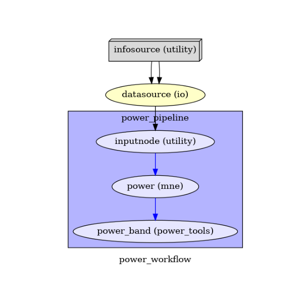
To do so, we first write the workflow graph (optional)

main_workflow.write_graph(graph2use='colored')  # colored

'/home/pasca/Tools/python/packages/neuropycon/ephypype/examples/sample_BIDS_omega/power_workflow/graph.png'

and visualize it. Take a moment to pause and notice how the connections here correspond to how we connected the nodes.

import matplotlib.pyplot as plt  # noqa
img = plt.imread(op.join(data_path, power_analysis_name, 'graph.png'))
plt.figure(figsize=(6, 6))
plt.imshow(img)
plt.axis('off')

(-0.5, 404.5, 498.5, -0.5)

Finally, we are now ready to execute our workflow.

main_workflow.config['execution'] = {'remove_unnecessary_outputs': 'false'}

# Run workflow locally on 1 CPU
main_workflow.run(plugin='MultiProc', plugin_args={'n_procs': NJOBS})

<networkx.classes.digraph.DiGraph object at 0x7fdf878c6110>

The outputs are the psd tensor and frequencies in .npz format and the mean PSD in .npy format stored in the workflow directory defined by base_dir

Note

The power pipeline in the source space is implemented by the function ephypype.pipelines.power.create_pipeline_power_src_space() and its Node ephypype.interfaces.mne.power.Power compute the PSD by the welch function of the scipy package.

from ephypype.gather import get_results  # noqa
from visbrain.objects import SourceObj, SceneObj, ColorbarObj  # noqa
from visbrain.utils import normalize  # noqa
from nipype.utils.filemanip import split_filename  # noqa

psd_files, channel_coo_files = get_results(main_workflow.base_dir,
                                           main_workflow.name,
                                           pipeline='power')

sc = SceneObj(size=(1800, 500), bgcolor=(.1, .1, .1))
for psd_file, channel_coo_file in zip(psd_files, channel_coo_files):
    path_xyz, basename, ext = split_filename(psd_file)

    arch = np.load(psd_file)
    psds, freqs = arch['psds'], arch['freqs']
    xyz = np.genfromtxt(channel_coo_file, dtype=float)
    freq_bands = np.asarray(freq_bands)
    clim = (psds.min(), psds.max())
    cmap = 'cool'
    txtcolor = 'white'

    # Find indices of frequencies :
    idx_fplt = np.abs((freqs.reshape(1, 1, -1) -
                       freq_bands[..., np.newaxis])).argmin(2)
    psdf = np.array([psds[:, k[0]:k[1]].mean(1) for k in idx_fplt])
    radius = normalize(np.c_[psdf.min(1), psdf.max(1)], 5, 25).astype(float)

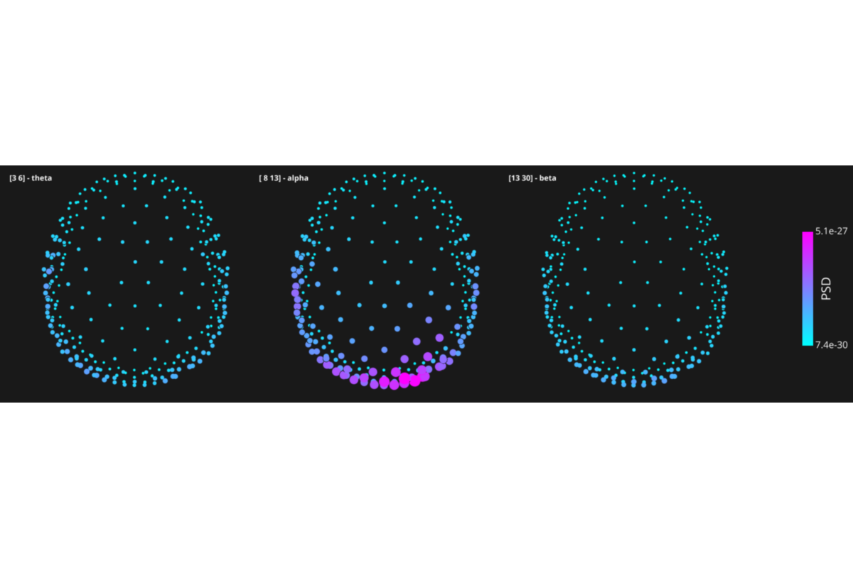
    for num, (fb, fbn, psd, rx) in enumerate(zip(freq_bands, freq_band_names,
                                                 psdf, radius)):
        s_obj = SourceObj('s', xyz, data=psd, radius_min=rx[0], radius_max=rx[1])  # noqa
        s_obj.color_sources(data=psd, cmap=cmap, clim=clim)
        sc.add_to_subplot(s_obj, col=num, title=str(fb) + ' - ' + fbn,
                          title_color=txtcolor, rotate='top', zoom=.6)
    cbar = ColorbarObj(s_obj, txtcolor=txtcolor, cblabel='PSD', txtsz=15,
                       cbtxtsz=20)
    sc.add_to_subplot(cbar, col=len(freq_bands), width_max=200)

sc.preview()