Compute connectivity on sensor space

The connectivity pipeline performs connectivity analysis in sensor or source space.

The input data should be a time series matrix in npy or mat format.

# Authors: Annalisa Pascarella <a.pascarella@iac.cnr.it>
# License: BSD (3-clause)

# sphinx_gallery_thumbnail_number = 2

import os.path as op
import numpy as np
import nipype.pipeline.engine as pe

import ephypype
from ephypype.nodes import create_iterator, create_datagrabber
from ephypype.nodes import get_frequency_band
from ephypype.datasets import fetch_omega_dataset

Let us fetch the data first. It is around 675 MB download.

base_path = op.join(op.dirname(ephypype.__file__), '..', 'examples')
data_path = fetch_omega_dataset(base_path)

then read the parameters for experiment and connectivity from a json file and print it

import json  # noqa
import pprint  # noqa
params = json.load(open("params.json"))

pprint.pprint({'experiment parameters': params["general"]})
subject_ids = params["general"]["subject_ids"]  # sub-003
session_ids = params["general"]["session_ids"]  # ses-0001
NJOBS = params["general"]["NJOBS"]

pprint.pprint({'connectivity parameters': params["connectivity"]})
freq_band_names = params["connectivity"]['freq_band_names']
freq_bands = params["connectivity"]['freq_bands']
con_method = params["connectivity"]['method']
epoch_window_length = params["connectivity"]['epoch_window_length']

{'experiment parameters': {'NJOBS': 1,
                           'data_type': 'fif',
                           'session_ids': ['ses-0001'],
                           'subject_ids': ['sub-0003'],
                           'subjects_dir': 'FSF'}}
{'connectivity parameters': {'epoch_window_length': 3.0,
                             'freq_band_names': ['alpha', 'beta'],
                             'freq_bands': [[8, 12], [13, 29]],
                             'method': 'coh'}}

Then, we create our workflow and specify the base_dir which tells nipype the directory in which to store the outputs.

# workflow directory within the `base_dir`
correl_analysis_name = 'spectral_connectivity_' + con_method

main_workflow = pe.Workflow(name=correl_analysis_name)
main_workflow.base_dir = data_path

Then we create a node to pass input filenames to DataGrabber from nipype

infosource = create_iterator(['subject_id', 'session_id', 'freq_band_name'],
                             [subject_ids, session_ids, freq_band_names])

and a node to grab data. The template_args in this node iterate upon the values in the infosource node

template_path = '*%s/%s/meg/%s*rest*0_60*ica.fif'
template_args = [['subject_id', 'session_id', 'subject_id']]
datasource = create_datagrabber(data_path, template_path, template_args)

Ephypype creates for us a pipeline which can be connected to these nodes we created. The connectivity pipeline is implemented by the function ephypype.pipelines.ts_to_conmat.create_pipeline_time_series_to_spectral_connectivity(), thus to instantiate this connectivity pipeline node, we import it and pass our parameters to it. The connectivity pipeline contains two nodes and is based on the MNE Python functions computing frequency- and time-frequency-domain connectivity measures. A list of the different connectivity measures implemented by MNE can be found in the description of mne.viz.plot_connectivity_circle()

In particular, the two nodes are:

• ephypype.interfaces.mne.spectral.SpectralConn computes spectral connectivity in a given frequency bands

• ephypype.interfaces.mne.spectral.PlotSpectralConn plot connectivity matrix using the spectral_connectivity function function

from ephypype.pipelines import create_pipeline_time_series_to_spectral_connectivity # noqa
spectral_workflow = create_pipeline_time_series_to_spectral_connectivity(
    data_path, con_method=con_method,
    epoch_window_length=epoch_window_length)

$$$$$$$$$$$$$$$$$$$$$$$$ Multiple trials $$$$$$$$$$$$$$$$$$$$$

The connectivity node needs two auxiliary nodes: one node reads the raw data file in .fif format and extract the data and the channel information; the other node get information on the frequency band we are interested on.

from ephypype.nodes.import_data import Fif2Array  # noqa
create_array_node = pe.Node(interface=Fif2Array(), name='Fif2Array')

frequency_node = get_frequency_band(freq_band_names, freq_bands)

We then connect the nodes two at a time. First, we connect two outputs (subject_id and session_id) of the infosource node to the datasource node. So, these two nodes taken together can grab data. The third output of infosource (freq_band_name) is connected to the frequency node

main_workflow.connect(infosource, 'subject_id', datasource, 'subject_id')
main_workflow.connect(infosource, 'session_id', datasource, 'session_id')

main_workflow.connect(infosource, 'freq_band_name',
                      frequency_node, 'freq_band_name')

Similarly, for the inputnode of create_array_node and spectral_workflow. Things will become clearer in a moment when we plot the graph of the workflow

main_workflow.connect(datasource, 'raw_file',
                      create_array_node, 'fif_file')
main_workflow.connect(create_array_node, 'array_file',
                      spectral_workflow, 'inputnode.ts_file')
main_workflow.connect(create_array_node, 'channel_names_file',
                      spectral_workflow, 'inputnode.labels_file')
main_workflow.connect(frequency_node, 'freq_bands',
                      spectral_workflow, 'inputnode.freq_band')
main_workflow.connect(create_array_node, 'sfreq',
                      spectral_workflow, 'inputnode.sfreq')

To do so, we first write the workflow graph (optional)

main_workflow.write_graph(graph2use='colored')  # colored

'/home/pasca/Tools/python/packages/neuropycon/ephypype/examples/sample_BIDS_omega/spectral_connectivity_coh/graph.png'

and visualize it. Take a moment to pause and notice how the connections here correspond to how we connected the nodes.

import matplotlib.pyplot as plt  # noqa
img = plt.imread(op.join(data_path, correl_analysis_name, 'graph.png'))
plt.figure(figsize=(8, 8))
plt.imshow(img)
plt.axis('off')

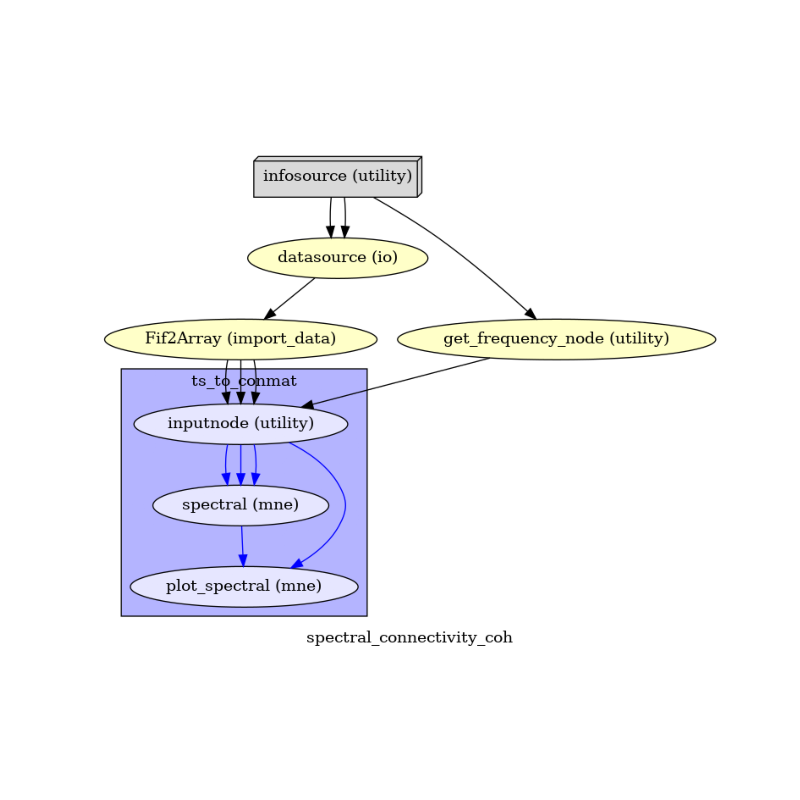
(-0.5, 732.5, 594.5, -0.5)

Finally, we are now ready to execute our workflow.

main_workflow.config['execution'] = {'remove_unnecessary_outputs': 'false'}

# Run workflow locally on 1 CPU
main_workflow.run(plugin='MultiProc', plugin_args={'n_procs': NJOBS})

<networkx.classes.digraph.DiGraph object at 0x7fdf1c791720>

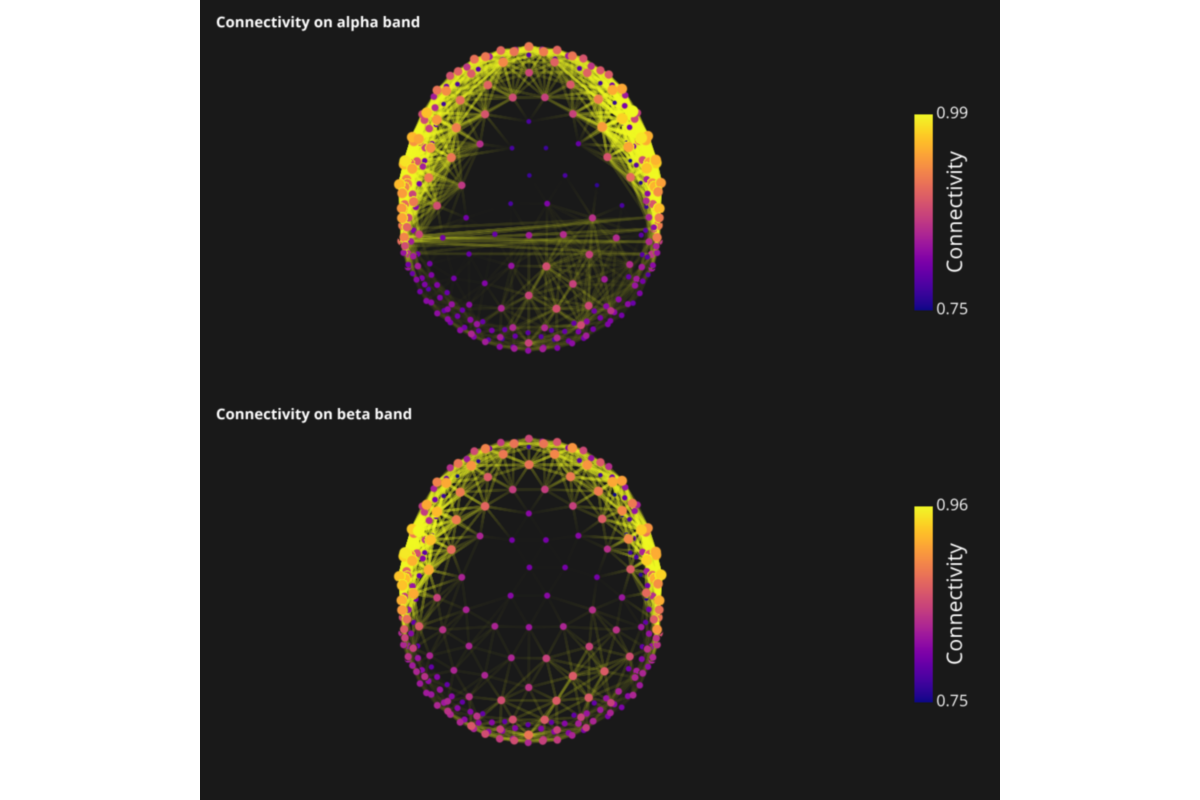
The output is the spectral connectivty matrix in .npy format stored in the workflow directory defined by base_dir. We can use the pipelines defined in graphpype package to perform graph analysis on the computed connectivity matrix.

from ephypype.gather import get_results  # noqa
from ephypype.gather import get_channel_files  # noqa
from ephypype.aux_tools import _parse_string  # noqa
from visbrain.objects import ConnectObj, SourceObj, SceneObj, ColorbarObj  # noqa

thresh = .75
with_text = False

channel_coo_files, channel_name_files = get_channel_files(
        main_workflow.base_dir, main_workflow.name)

connectivity_matrices, _ = get_results(
        main_workflow.base_dir, main_workflow.name, pipeline='connectivity')

sc = SceneObj(size=(1000, 1000), bgcolor=(.1, .1, .1))
for nf, (connect_file, channel_coo_file, channel_name_file) in \
        enumerate(zip(connectivity_matrices, channel_coo_files,
                      channel_name_files)):

    # Load files :
    xyz = np.genfromtxt(channel_coo_file, dtype=float)
    names = np.genfromtxt(channel_name_file, dtype=str)
    connect = np.load(connect_file)
    connect += connect.T
    connect = np.ma.masked_array(connect, mask=connect < thresh)
    names = names if with_text else None
    radius = connect.sum(1)
    clim = (thresh, connect.max())
    cmap = 'plasma'
    txtcolor = 'white'

    # With text :
    c_obj = ConnectObj('c', xyz, connect,
                       color_by='count',
                       clim=clim, dynamic=(0., 1.),
                       dynamic_order=3, antialias=True, cmap=cmap,
                       line_width=4.)
    s_obj = SourceObj('s', xyz, data=radius, radius_min=5, radius_max=15,
                      text=names, text_size=10, text_color=txtcolor,
                      text_translate=(0., 0., 0.))
    s_obj.color_sources(data=radius, cmap=cmap)
    cbar = ColorbarObj(c_obj, txtcolor=txtcolor, txtsz=15,
                       cblabel='Connectivity', cbtxtsz=20)
    band = _parse_string(connect_file, freq_band_names)
    title = 'Connectivity on {} band'.format(band)
    sc.add_to_subplot(c_obj, title=title, title_size=14, title_bold=True,
                      title_color=txtcolor, row=nf)
    sc.add_to_subplot(s_obj, rotate='top', zoom=.5, use_this_cam=True, row=nf)
    sc.add_to_subplot(cbar, col=1, width_max=200, row=nf)

sc.preview()