Compute Graph properties from a given connectivity matrix with BCT toolbox¶

The _inv_ts_to_bct_graph pipeline performs spectral connectivity over time series, and an example wrap of a function from the Brain Connectivity Toolbox as an alternative to the Radatools toolbox for graph metric computation.

This workflow makes use of two chained pipelines, and requires both graphpype AND ephypype to be installed.

The input data should be a time series matrix in npy format.

# Authors: David Meunier <david_meunier_79@hotmail.fr>
# License: BSD (3-clause)
# sphinx_gallery_thumbnail_number = 2
import os.path as op
import nipype.pipeline.engine as pe
import nipype.interfaces.io as nio

from ephypype.nodes import create_iterator
from ephypype.nodes import get_frequency_band

Check if data are available

from graphpype.utils_tests import load_test_data

data_path = load_test_data("data_inv_ts")

First, we create our workflow and specify the base_dir which tells nipype the directory in which to store the outputs.

# workflow directory within the `base_dir`
graph_analysis_name = 'inv_ts_to_graph_analysis'

main_workflow = pe.Workflow(name=graph_analysis_name)
main_workflow.base_dir = data_path

We now use a json file for describing the connectivity parameters, loaded from a json as a dictionnary

import json  # noqa
import pprint  # noqa

data_con = json.load(open(op.join(op.dirname("__file__"),
                                  "params_connectivity.json")))
pprint.pprint({'connectivity parameters': data_con})

freq_band_names = data_con['freq_band_names']
freq_bands = data_con['freq_bands']

# spectral_connectivity_parameters
con_method = data_con['con_method']
epoch_window_length = data_con['epoch_window_length']

# sampling frequency
sfreq = data_con['sfreq'] # When starting from raw MEG
# (.fif) data, can be directly extracted from the file info

frequency_node = get_frequency_band(freq_band_names, freq_bands)

Out:

{'connectivity parameters': {'con_method': 'coh',
                             'epoch_window_length': 3.0,
                             'freq_band_names': ['alpha', 'beta'],
                             'freq_bands': [[8, 12], [13, 29]],
                             'sfreq': 2400}}

Then we create a node to pass input filenames to DataGrabber from nipype

subject_ids = ['sub-0003']  # 'sub-0004', 'sub-0006'
infosource = create_iterator(['subject_id', 'freq_band_name'],
                             [subject_ids, freq_band_names])

and a node to grab data. The template_args in this node iterate upon the values in the infosource node

template_path = '*%s_task-rest_run-01_meg_0_60_raw_filt_dsamp_ica_ROI_ts.npy'

datasource = pe.Node(
    interface=nio.DataGrabber(infields=['subject_id'], outfields=['ts_file']),
    name='datasource')

datasource.inputs.base_directory = data_path
datasource.inputs.template = template_path

datasource.inputs.template_args = dict(ts_file=[['subject_id']])
datasource.inputs.sort_filelist = True

We then use the pipeline used in the previous example conmat_to_graph pipeline

from ephypype.pipelines import create_pipeline_time_series_to_spectral_connectivity # noqa

spectral_workflow = create_pipeline_time_series_to_spectral_connectivity(
    data_path, con_method=con_method,
    epoch_window_length=epoch_window_length)

Out:

$$$$$$$$$$$$$$$$$$$$$$$$ Multiple trials $$$$$$$$$$$$$$$$$$$$$

We now use a json file for describing the graph parameters, loaded from a json as a dictionnary

data_graph = json.load(open(op.join(op.dirname("__file__"),
                                  "params_bct_graph.json")))
pprint.pprint({'graph parameters': data_graph})

# density of the threshold
con_den = data_graph['con_den']


from graphpype.pipelines import create_pipeline_bct_graph

graph_workflow = create_pipeline_bct_graph(
    data_path, con_den=con_den)

Out:

{'graph parameters': {'con_den': 0.05}}

We then connect the nodes two at a time. We connect the output of the infosource node to the datasource node. So, these two nodes taken together can grab data.

main_workflow.connect(infosource, 'subject_id',
                      datasource, 'subject_id')

main_workflow.connect(infosource, 'freq_band_name',
                      frequency_node, 'freq_band_name')

main_workflow.connect(datasource, 'ts_file',
                      spectral_workflow, "inputnode.ts_file")

spectral_workflow.inputs.inputnode.sfreq = sfreq

main_workflow.connect(frequency_node, 'freq_bands',
                      spectral_workflow, 'inputnode.freq_band')

main_workflow.connect(spectral_workflow, 'spectral.conmat_file',
                      graph_workflow, "inputnode.conmat_file")

To do so, we first write the workflow graph (optional)

main_workflow.write_graph(graph2use='colored')  # colored

and visualize it. Take a moment to pause and notice how the connections correspond to how we connected the nodes.

#import matplotlib.pyplot as plt  # noqa
#img = plt.imread(op.join(data_path, graph_analysis_name, 'graph.png'))
#plt.figure(figsize=(8, 8))
#plt.imshow(img)
#plt.axis('off')
#plt.show()

Finally, we are now ready to execute our workflow.

main_workflow.config['execution'] = {'remove_unnecessary_outputs': 'false'}
main_workflow.run()

Run workflow locally on 2 CPUs in parrallel main_workflow.run(plugin=’MultiProc’, plugin_args={‘n_procs’: 2}) ###############################################################################

plotting k_core values

#from graphpype.utils_visbrain import visu_graph # noqa

#labels_file = op.join(data_path, "label_names.txt")
#coords_file = op.join(data_path, "label_centroid.txt")

##labels_file = op.join(data_path, "label_names.txt")
##coords_file = op.join(data_path, "label_centroid.txt")

#from visbrain.objects import SceneObj, BrainObj # noqa

#sc = SceneObj(size=(1500, 1500), bgcolor=(1,1,1))

#views = ["left",'top']


#for nf, freq_band_name in enumerate(freq_band_names):

    #res_path = op.join(
        #data_path, graph_analysis_name,
        #"graph_bct_pipe",
        #"_freq_band_name_"+freq_band_name+"_subject_id_sub-0003")

    #node_k_file = op.join(res_path, "k_core", "coreness.npy")

    #bin_mat_file = op.join(res_path, "bin_mat", "bin_mat.npy")

    #for i_v,view in enumerate(views):
        #b_obj = BrainObj('B1', translucent=True)

        #sc.add_to_subplot(b_obj, row=nf, col = i_v, use_this_cam=True, rotate=view,
                        #title=("K-core nodes for {} band".format(freq_band_name)),
                        #title_size=14, title_bold=True, title_color='black')

        #c_obj,s_obj = visu_graph(
            #labels_file = labels_file, coords_file = coords_file,
            ##net_file = bin_mat_file)
            #net_file = bin_mat_file, node_size_file=node_k_file)

        #sc.add_to_subplot(c_obj, row=nf, col = i_v)
        #sc.add_to_subplot(s_obj, row=nf, col = i_v)

#sc.preview()

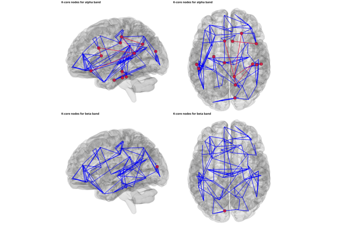
plotting k_core only

from graphpype.utils_visbrain import visu_graph_kcore # noqa

labels_file = op.join(data_path, "label_names.txt")
coords_file = op.join(data_path, "label_centroid.txt")

#labels_file = op.join(data_path, "label_names.txt")
#coords_file = op.join(data_path, "label_centroid.txt")

from visbrain.objects import SceneObj, BrainObj # noqa

sc = SceneObj(size=(1500, 1500), bgcolor=(1,1,1))

views = ["left",'top']


for nf, freq_band_name in enumerate(freq_band_names):

    res_path = op.join(
        data_path, graph_analysis_name,
        "graph_bct_pipe",
        "_freq_band_name_"+freq_band_name+"_subject_id_sub-0003")

    node_k_file = op.join(res_path, "k_core", "coreness.npy")

    bin_mat_file = op.join(res_path, "bin_mat", "bin_mat.npy")

    for i_v,view in enumerate(views):
        b_obj = BrainObj('B1', translucent=True)

        sc.add_to_subplot(b_obj, row=nf, col = i_v, use_this_cam=True, rotate=view,
                        title=("K-core nodes for {} band".format(freq_band_name)),
                        title_size=14, title_bold=True, title_color='black')

        c_obj,s_obj, c_obj2, s_obj2,  = visu_graph_kcore(
            labels_file = labels_file, coords_file = coords_file,
            #net_file = bin_mat_file)
            net_file = bin_mat_file, node_size_file=node_k_file)

        sc.add_to_subplot(c_obj, row=nf, col = i_v)
        sc.add_to_subplot(s_obj, row=nf, col = i_v)

        if c_obj2:
            sc.add_to_subplot(c_obj2, row=nf, col = i_v)

        sc.add_to_subplot(s_obj2, row=nf, col = i_v)


sc.preview()

../_images/sphx_glr_plot_inv_ts_to_bct_graph_001.png

Total running time of the script: ( 0 minutes 5.839 seconds)

Gallery generated by Sphinx-Gallery