Compute Graph properties from a given connectivity matrix¶

The inv_ts_to_graph pipeline performs spectral connectivity and graph analysis over time series. This workflow makes use of two chained pipelines, and requires both graphpype AND ephypype to be installed.

The input data should be a time series matrix in npy format.

# Authors: David Meunier <david_meunier_79@hotmail.fr>
# License: BSD (3-clause)
# sphinx_gallery_thumbnail_number = 2
import os.path as op
import nipype.pipeline.engine as pe
import nipype.interfaces.io as nio

from ephypype.nodes import create_iterator
from ephypype.nodes import get_frequency_band

Check if data are available

from graphpype.utils_tests import load_test_data

data_path = load_test_data("data_inv_ts")

First, we create our workflow and specify the base_dir which tells nipype the directory in which to store the outputs.

# workflow directory within the `base_dir`
graph_analysis_name = 'inv_ts_to_graph_analysis'

main_workflow = pe.Workflow(name=graph_analysis_name)
main_workflow.base_dir = data_path

We now use a json file for describing the connectivity parameters, loaded from a json as a dictionnary

import json  # noqa
import pprint  # noqa

data_con = json.load(open(op.join(op.dirname("__file__"),
                                  "params_connectivity.json")))
pprint.pprint({'connectivity parameters': data_con})

freq_band_names = data_con['freq_band_names']
freq_bands = data_con['freq_bands']

# spectral_connectivity_parameters
con_method = data_con['con_method']
epoch_window_length = data_con['epoch_window_length']

# sampling frequency
sfreq = data_con['sfreq'] # When starting from raw MEG
# (.fif) data, can be directly extracted from the file info

frequency_node = get_frequency_band(freq_band_names, freq_bands)

Out:

{'connectivity parameters': {'con_method': 'coh',
                             'epoch_window_length': 3.0,
                             'freq_band_names': ['alpha', 'beta'],
                             'freq_bands': [[8, 12], [13, 29]],
                             'sfreq': 2400}}

Then we create a node to pass input filenames to DataGrabber from nipype

subject_ids = ['sub-0003']  # 'sub-0004', 'sub-0006'
infosource = create_iterator(['subject_id', 'freq_band_name'],
                             [subject_ids, freq_band_names])

and a node to grab data. The template_args in this node iterate upon the values in the infosource node

template_path = '*%s_task-rest_run-01_meg_0_60_raw_filt_dsamp_ica_ROI_ts.npy'

datasource = pe.Node(
    interface=nio.DataGrabber(infields=['subject_id'], outfields=['ts_file']),
    name='datasource')

datasource.inputs.base_directory = data_path
datasource.inputs.template = template_path

datasource.inputs.template_args = dict(ts_file=[['subject_id']])
datasource.inputs.sort_filelist = True

We then use the pipeline used in the previous example conmat_to_graph pipeline

from ephypype.pipelines import create_pipeline_time_series_to_spectral_connectivity # noqa

spectral_workflow = create_pipeline_time_series_to_spectral_connectivity(
    data_path, con_method=con_method,
    epoch_window_length=epoch_window_length)

Out:

$$$$$$$$$$$$$$$$$$$$$$$$ Multiple trials $$$$$$$$$$$$$$$$$$$$$

We now use a json file for describing the graph parameters, loaded from a json as a dictionnary

data_graph = json.load(open(op.join(op.dirname("__file__"),
                                  "params_graph.json")))
pprint.pprint({'graph parameters': data_graph})

# density of the threshold. This parameter corrdesponds to the percentage of
# highest connections retains for the analyses. con_den = 1.0 means a fully
# connected graphs (all edges are present)

con_den = data_graph['con_den']

# The optimisation sequence
radatools_optim = data_graph['radatools_optim']

Out:

{'graph parameters': {'con_den': 0.05, 'radatools_optim': 'WN tfrf 100'}}

see http://deim.urv.cat/~sergio.gomez/download.php?f=radatools-5.0-README.txt for more details, but very briefly:

1. WN for weighted unsigned (typically coherence, pli, etc.) and WS for signed (e.g. Pearson correlation)
1. the optimisation sequence, can be used in different order. The sequence tfrf is proposed in radatools, and means: t = tabu search , f = fast algorithm, r = reposition algorithm and f = fast algorithm (again)
1. the last number is the number of repetitions of the algorithm, out of which the best one is chosen. The higher the number of repetitions, the higher the chance to reach the global maximum, but also the longer the computation takes. For testing, 1 is admissible, but it is expected to have at least 100 is required for reliable results

Graphpype creates for us a graph pipeline, implemented by the function :func: graphpype.pipelines.conmat_to_graph.create_pipeline_conmat_to_graph_density ,thus to instantiate this graph pipeline node, we import it and pass our parameters to it.

The graph pipeline contains several nodes, some are based on radatools

Two nodes of particular interest are :

graphpype.interfaces.radatools.rada.CommRada computes Community detection based on the previous radatools_optim parameters
graphpype.interfaces.radatools.rada.NetPropRada computes most of the classical graph-based metrics (Small-World, Efficiency, Assortativity, etc.)

from graphpype.pipelines import create_pipeline_conmat_to_graph_density

graph_workflow = create_pipeline_conmat_to_graph_density(
    data_path, con_den=con_den, optim_seq=radatools_optim)

We then connect the nodes two at a time. We connect the output of the infosource node to the datasource node. So, these two nodes taken together can grab data.

main_workflow.connect(infosource, 'subject_id',
                      datasource, 'subject_id')

main_workflow.connect(infosource, 'freq_band_name',
                      frequency_node, 'freq_band_name')

main_workflow.connect(datasource, 'ts_file',
                      spectral_workflow, "inputnode.ts_file")

spectral_workflow.inputs.inputnode.sfreq = sfreq

main_workflow.connect(frequency_node, 'freq_bands',
                      spectral_workflow, 'inputnode.freq_band')

main_workflow.connect(spectral_workflow, 'spectral.conmat_file',
                      graph_workflow, "inputnode.conmat_file")

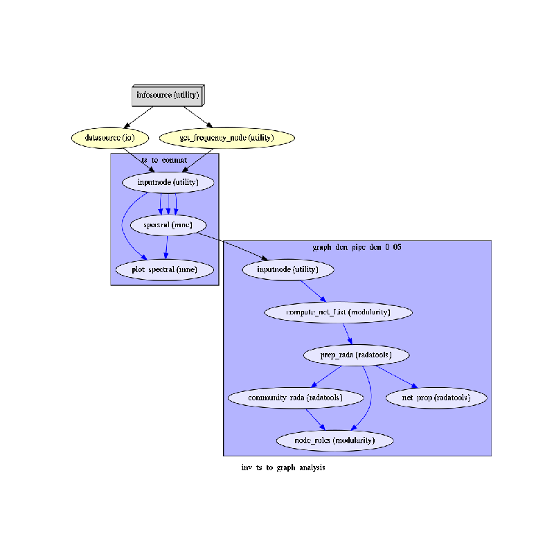
To do so, we first write the workflow graph (optional)

main_workflow.write_graph(graph2use='colored')  # colored

and visualize it. Take a moment to pause and notice how the connections correspond to how we connected the nodes.

import matplotlib.pyplot as plt  # noqa
img = plt.imread(op.join(data_path, graph_analysis_name, 'graph.png'))
plt.figure(figsize=(8, 8))
plt.imshow(img)
plt.axis('off')
plt.show()

../_images/sphx_glr_plot_inv_ts_to_graph_001.png

Finally, we are now ready to execute our workflow.

main_workflow.config['execution'] = {'remove_unnecessary_outputs': 'false'}

Run workflow locally on 2 CPUs in parrallel main_workflow.run(plugin=’MultiProc’, plugin_args={‘n_procs’: 2})

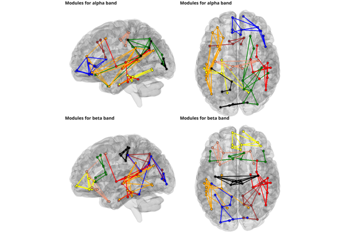
plotting modules

from graphpype.utils_visbrain import visu_graph_modules # noqa

labels_file = op.join(data_path, "label_names.txt")
coords_file = op.join(data_path, "label_centroid.txt")

from visbrain.objects import SceneObj, BrainObj # noqa

sc = SceneObj(size=(1000, 1000), bgcolor=(1,1,1))

views = ["left",'top']

for i_v,view in enumerate(views):
    for nf, freq_band_name in enumerate(freq_band_names):
        res_path = op.join(
            data_path, graph_analysis_name,
            "graph_den_pipe_den_"+str(con_den).replace(".", "_"),
            "_freq_band_name_"+freq_band_name+"_subject_id_sub-0003")

        lol_file = op.join(res_path, "community_rada", "Z_List.lol")
        net_file = op.join(res_path, "prep_rada", "Z_List.net")

        b_obj = BrainObj("B1", translucent=True)
        sc.add_to_subplot(b_obj, row=nf, col = i_v, use_this_cam=True,
                          rotate=view,
                          title=("Modules for {} band".format(freq_band_name)),
                          title_size=14, title_bold=True, title_color='black')


        c_obj,s_obj = visu_graph_modules(lol_file=lol_file, net_file=net_file,
                                coords_file=coords_file,
                                inter_modules=False)

        sc.add_to_subplot(c_obj, row=nf, col = i_v)
        sc.add_to_subplot(s_obj, row=nf, col = i_v)

sc.preview()

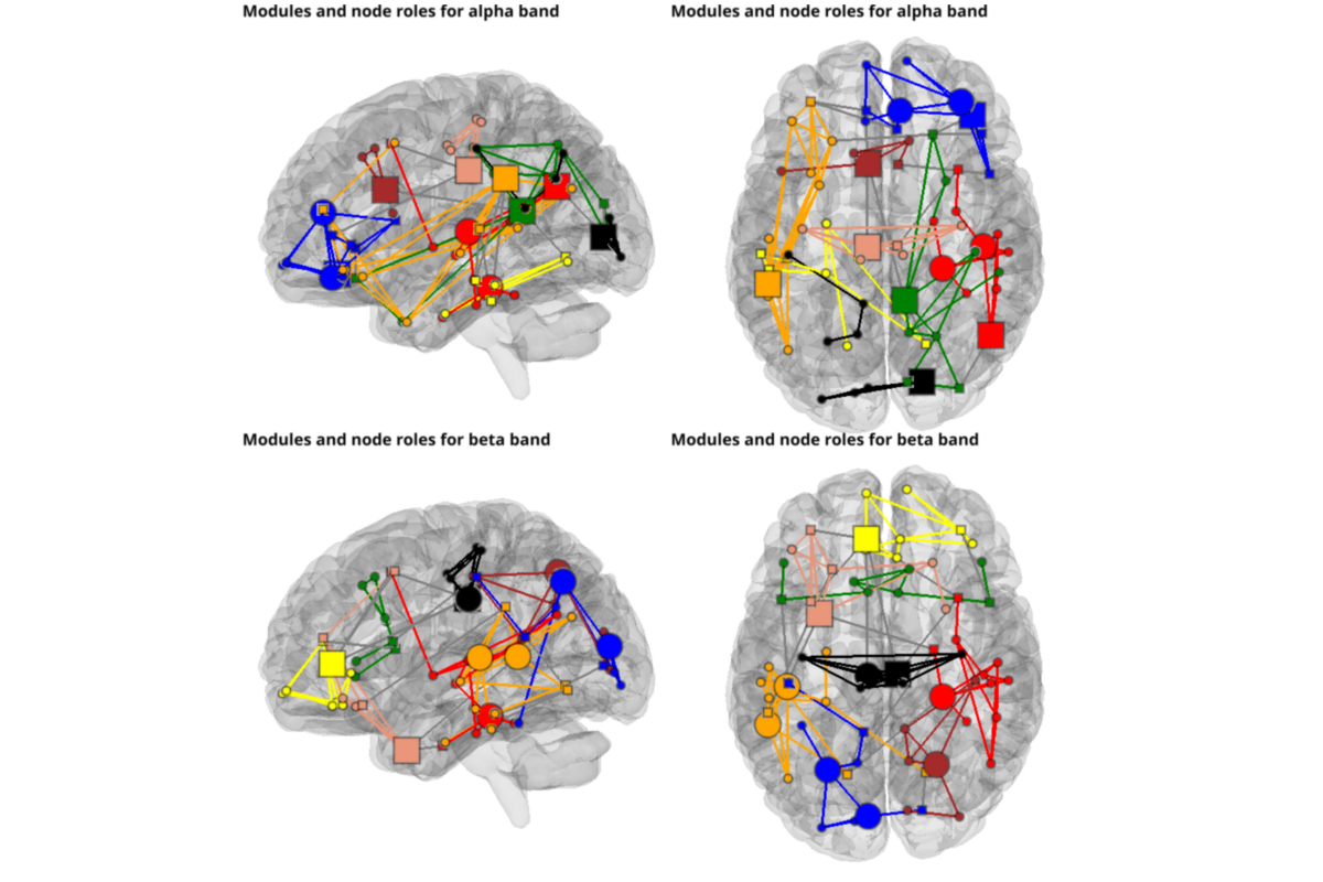
../_images/sphx_glr_plot_inv_ts_to_graph_002.png

plotting modules and roles

from graphpype.utils_visbrain import visu_graph_modules_roles # noqa

labels_file = op.join(data_path, "label_names.txt")
coords_file = op.join(data_path, "label_centroid.txt")

from visbrain.objects import SceneObj, BrainObj # noqa

sc = SceneObj(size=(1000, 1000), bgcolor=(1,1,1))

views = ["left",'top']


for nf, freq_band_name in enumerate(freq_band_names):

    res_path = op.join(
        data_path, graph_analysis_name,
        "graph_den_pipe_den_"+str(con_den).replace(".", "_"),
        "_freq_band_name_"+freq_band_name+"_subject_id_sub-0003")

    lol_file = op.join(res_path, "community_rada", "Z_List.lol")
    net_file = op.join(res_path, "prep_rada", "Z_List.net")
    roles_file = op.join(res_path, "node_roles", "node_roles.txt")

    for i_v,view in enumerate(views):
        b_obj = BrainObj('B1', translucent=True)

        sc.add_to_subplot(b_obj, row=nf, col = i_v, use_this_cam=True, rotate=view,
                        title=("Modules and node roles for {} band".format(freq_band_name)),
                        title_size=14, title_bold=True, title_color='black')

        c_obj,list_sources = visu_graph_modules_roles(
            lol_file=lol_file, net_file=net_file, roles_file=roles_file,
            coords_file=coords_file, inter_modules=True, default_size=10,
            hub_to_non_hub=3)

        sc.add_to_subplot(c_obj, row=nf, col = i_v)

        for source in list_sources:
            sc.add_to_subplot(source, row=nf, col = i_v)

sc.preview()

../_images/sphx_glr_plot_inv_ts_to_graph_003.png

Total running time of the script: ( 0 minutes 5.431 seconds)

Gallery generated by Sphinx-Gallery