Compute inverse solution

The inverse solution pipeline performs source reconstruction starting either from raw/epoched data (.fif format) specified by the user or from the output of the Preprocessing pipeline (cleaned raw data).

# Authors: Annalisa Pascarella <a.pascarella@iac.cnr.it>
# License: BSD (3-clause)

# sphinx_gallery_thumbnail_number = 2

import os.path as op
import numpy as np
import nipype.pipeline.engine as pe
import nipype.interfaces.io as nio

import ephypype
from ephypype.nodes import create_iterator
from ephypype.datasets import fetch_omega_dataset

Let us fetch the data first. It is around 675 MB download.

base_path = op.join(op.dirname(ephypype.__file__), '..', 'examples')
data_path = fetch_omega_dataset(base_path)

then read the parameters for experiment and inverse problem from a json file and print it

import json  # noqa
import pprint  # noqa
params = json.load(open("params.json"))

pprint.pprint({'experiment parameters': params["general"]})
subject_ids = params["general"]["subject_ids"]  # sub-003
session_ids = params["general"]["session_ids"]  # ses-0001
NJOBS = params["general"]["NJOBS"]

pprint.pprint({'inverse parameters': params["inverse"]})
spacing = params["inverse"]['spacing']  # ico-5 vs oct-6
snr = params["inverse"]['snr']  # use smaller SNR for raw data
inv_method = params["inverse"]['img_method']  # sLORETA, MNE, dSPM, LCMV
parc = params["inverse"]['parcellation']  # parcellation to use: 'aparc' vs 'aparc.a2009s'  # noqa
# noise covariance matrix filename template
noise_cov_fname = params["inverse"]['noise_cov_fname']

# set sbj dir path, i.e. where the FS folfers are
subjects_dir = op.join(data_path, params["general"]["subjects_dir"])

{'experiment parameters': {'NJOBS': 1,
                           'data_type': 'fif',
                           'session_ids': ['ses-0001'],
                           'subject_ids': ['sub-0003'],
                           'subjects_dir': 'FSF'}}
{'inverse parameters': {'img_method': 'MNE',
                        'method': 'LCMV',
                        'noise_cov_fname': '*noise*.ds',
                        'parcellation': 'aparc',
                        'snr': 1.0,
                        'spacing': 'oct-6'}}

Then, we create our workflow and specify the base_dir which tells nipype the directory in which to store the outputs.

# workflow directory within the `base_dir`
src_reconstruction_pipeline_name = 'source_reconstruction_' + \
    inv_method + '_' + parc.replace('.', '')

main_workflow = pe.Workflow(name=src_reconstruction_pipeline_name)
main_workflow.base_dir = data_path

Then we create a node to pass input filenames to DataGrabber from nipype

infosource = create_iterator(['subject_id', 'session_id'],
                             [subject_ids, session_ids])

and a node to grab data. The template_args in this node iterate upon the values in the infosource node

datasource = pe.Node(interface=nio.DataGrabber(infields=['subject_id'],
                                               outfields=['raw_file', 'trans_file']),  # noqa
                     name='datasource')

datasource.inputs.base_directory = data_path
datasource.inputs.template = '*%s/%s/meg/%s*rest*%s.fif'

datasource.inputs.template_args = dict(
        raw_file=[['subject_id', 'session_id', 'subject_id', '0_60*ica']],
        trans_file=[['subject_id', 'session_id', 'subject_id', "-trans"]])

datasource.inputs.sort_filelist = True

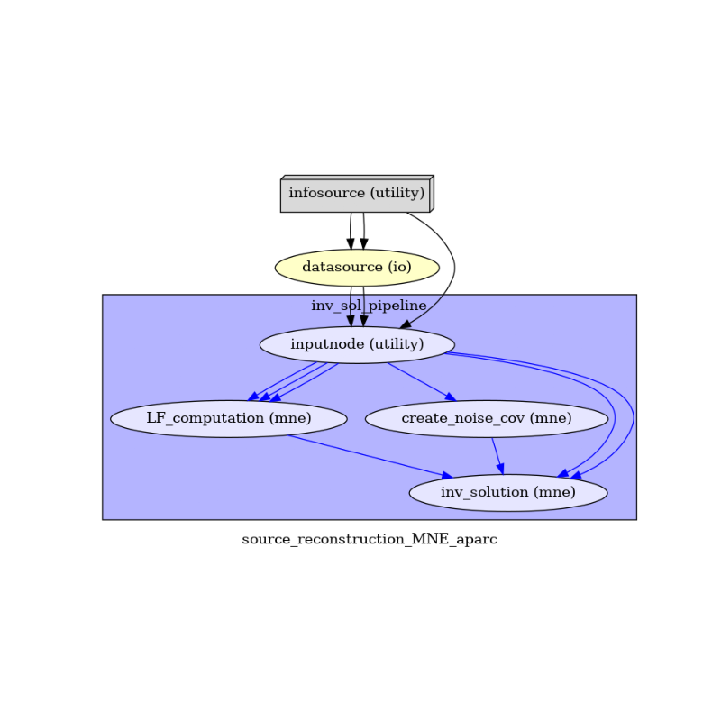
Ephypype creates for us a pipeline which can be connected to these nodes we created. The inverse solution pipeline is implemented by the function ephypype.pipelines.create_pipeline_source_reconstruction() thus to instantiate the inverse pipeline node, we import it and pass our parameters to it. The inverse pipeline contains three nodes that wrap the MNE Python functions that perform the source reconstruction steps.

In particular, the three nodes are:

• ephypype.interfaces.mne.LF_computation.LFComputation compute the Lead Field matrix

• ephypype.interfaces.mne.Inverse_solution.NoiseCovariance computes the noise covariance matrix

• ephypype.interfaces.mne.Inverse_solution.InverseSolution estimates the time series of the neural sources on a set of dipoles grid

from ephypype.pipelines import create_pipeline_source_reconstruction  # noqa
inv_sol_workflow = create_pipeline_source_reconstruction(
    data_path, subjects_dir, spacing=spacing, inv_method=inv_method, parc=parc,
    noise_cov_fname=noise_cov_fname)

******************** {} *noise*.ds

We then connect the nodes two at a time. First, we connect the two outputs (subject_id and session_id) of the infosource node to the datasource node. So, these two nodes taken together can grab data.

main_workflow.connect(infosource, 'subject_id', datasource, 'subject_id')
main_workflow.connect(infosource, 'session_id', datasource, 'session_id')

Similarly, for the inputnode of the preproc_workflow. Things will become clearer in a moment when we plot the graph of the workflow.

main_workflow.connect(infosource, 'subject_id',
                      inv_sol_workflow, 'inputnode.sbj_id')
main_workflow.connect(datasource, 'raw_file',
                      inv_sol_workflow, 'inputnode.raw')
main_workflow.connect(datasource, 'trans_file',
                      inv_sol_workflow, 'inputnode.trans_file')

To do so, we first write the workflow graph (optional)

main_workflow.write_graph(graph2use='colored')  # colored

'/home/pasca/Tools/python/packages/neuropycon/ephypype/examples/sample_BIDS_omega/source_reconstruction_MNE_aparc/graph.png'

and visualize it. Take a moment to pause and notice how the connections here correspond to how we connected the nodes.

import matplotlib.pyplot as plt  # noqa
img = plt.imread(op.join(data_path, src_reconstruction_pipeline_name, 'graph.png'))  # noqa
plt.figure(figsize=(8, 8))
plt.imshow(img)
plt.axis('off')

(-0.5, 724.5, 498.5, -0.5)

Finally, we are now ready to execute our workflow.

main_workflow.config['execution'] = {'remove_unnecessary_outputs': 'false'}

# Run workflow locally on 1 CPU
main_workflow.run(plugin='LegacyMultiProc', plugin_args={'n_procs': NJOBS})

<networkx.classes.digraph.DiGraph object at 0x7fdf1c7cc5b0>

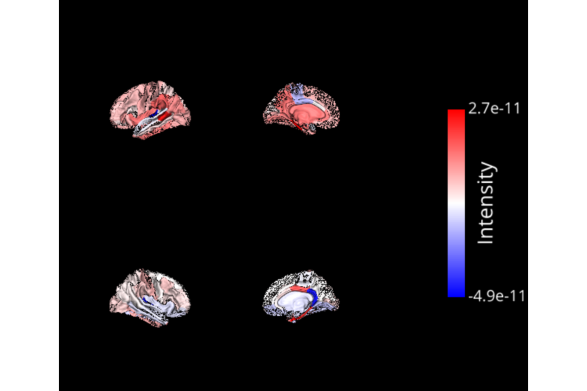
The output is the source reconstruction matrix stored in the workflow directory defined by base_dir. This matrix can be used as input of the Connectivity pipeline.

Warning

To use this pipeline, we need a cortical segmentation of MRI data, that could be provided by Freesurfer

import pickle  # noqa
from ephypype.gather import get_results  # noqa
from visbrain.objects import BrainObj, ColorbarObj, SceneObj  # noqa

time_series_files, label_files = get_results(main_workflow.base_dir,
                                             main_workflow.name,
                                             pipeline='inverse')

time_pts = 30

sc = SceneObj(size=(600, 500), bgcolor=(0, 0, 0))
lh_file = op.join(subjects_dir, 'fsaverage', 'label/lh.aparc.annot')
rh_file = op.join(subjects_dir, 'fsaverage', 'label/rh.aparc.annot')
cmap = 'bwr'
txtcolor = 'white'
for inverse_file, label_file in zip(time_series_files, label_files):
    # Load files :
    with open(label_file, 'rb') as f:
        ar = pickle.load(f)
        names, xyz, colors = ar['ROI_names'], ar['ROI_coords'], ar['ROI_colors']  # noqa
    ts = np.squeeze(np.load(inverse_file))
    cen = np.array([k.mean(0) for k in xyz])

    # Get the data of the left / right hemisphere :
    lh_data, rh_data = ts[::2, time_pts], ts[1::2, time_pts]
    clim = (ts[:, time_pts].min(), ts[:, time_pts].max())
    roi_names = [k[0:-3] for k in np.array(names)[::2]]

    # Left hemisphere outside :
    b_obj_li = BrainObj('white', translucent=False, hemisphere='left')
    b_obj_li.parcellize(lh_file, select=roi_names, data=lh_data, cmap=cmap)
    sc.add_to_subplot(b_obj_li, rotate='left')

    # Left hemisphere inside :
    b_obj_lo = BrainObj('white',  translucent=False, hemisphere='left')
    b_obj_lo.parcellize(lh_file, select=roi_names, data=lh_data, cmap=cmap)
    sc.add_to_subplot(b_obj_lo, col=1, rotate='right')

    # Right hemisphere outside :
    b_obj_ro = BrainObj('white',  translucent=False, hemisphere='right')
    b_obj_ro.parcellize(rh_file, select=roi_names, data=rh_data, cmap=cmap)
    sc.add_to_subplot(b_obj_ro, row=1, rotate='right')

    # Right hemisphere inside :
    b_obj_ri = BrainObj('white',  translucent=False, hemisphere='right')
    b_obj_ri.parcellize(rh_file, select=roi_names, data=rh_data, cmap=cmap)
    sc.add_to_subplot(b_obj_ri, row=1, col=1, rotate='left')

    # Add the colorbar :
    cbar = ColorbarObj(b_obj_li, txtsz=15, cbtxtsz=20, txtcolor=txtcolor,
                       cblabel='Intensity')
    sc.add_to_subplot(cbar, col=2, row_span=2)

sc.preview()